Investigating the Factors That Affect Real Estate Price's in California
Introduction
Housing prices are highly speculative. Expert price estimates tend to range greatly. The price of a house is seemingly dependent on so many variables that it can be difficult to extract what exactly is most important to look for. This analysis aims to find the primary variables that determine a house's sales price. The analysis will be run on a data set of approximately 1500 houses with over 60 different variables measured on each house. From this data set, my goal is to narrow down the important factors that affect a house's price.
The data used in this analysis is a Kaggle data set of the sales price of properties that includes 82 variables with 1459 observations. The data was curated for a Kaggle competition that investigates price estimation of homes depending on a variety of explanatory variables. The list of explanatory variables can be seen in the appendix.
My objective in this analysis is to identify the primary explanatory variables that affect the price of any given property given the explanatory variables. To achieve this I will be using multiple linear regression to obtain the important factors and end up with a model that can predict sales price with relatively high accuracy.
Method
The method I will use to estimate the property prices is multiple linear regression. However, the data needs to meet the assumptions to use multiple linear regression affectivly:
- The dependent variable should be measured on a continuos scale
- There must be a linear relationship between the dependent and independent variables
- The variance of the residuals should be equal at each level of the explanatory variables
- The errors must be independent from one another
- The risiduals must be normally distributed
- There should be no outliers or influential points
- There should be no multi collinearity
There are several ways to insure tha the data meets the given assumptions and this will be seen in the analysis section. Given that all asspects are met we can use Multiple linear regression to analyse the data. Multiple linear regression is an extension of linear regression, as it uses two or more explanatory variables. The method aims to use the explanatory or independent variables to estimate the dependent variable. In this case, our dependent variable is the property's sale price and the explanatory variables are a collection of measurements and observations made on the property.
Data Cleaning
The data set had several different quantitative variable types including continuos, discrete and categorical variables. As a linear regression only deals with numeric values, the categorical data needed to be converted into a numeric format. To do this I cast all the categorical variables to a numeric value based on their nature. For example, the condition of the over all house had 5 categorical variables ranging from horrible condition to excelent condition. Therefore, I cast each category to a number betweek 1 and 5 from bad to good. That being said some of the data found in the dataset was unfortunately unusable given that it was descriptive by nature and was open to interpretation. To keep the analysis relativly simple I cut out these variables. I used the following code snippet to transform the categorical variables into numeric variables.
df = pd.read_csv('train.csv')
df['LotShape'].iloc[df['LotShape'] == 'Reg'] = 0
df['LotShape'].iloc[df['LotShape'] == 'IR1'] = 1
df['LotShape'].iloc[df['LotShape'] == 'IR2'] = 2
df['LotShape'].iloc[df['LotShape'] == 'IR3'] = 3
df['LotShape']=df['LotShape'].astype(int)


df['ExterQual'].iloc[df['ExterQual'] == 'Ex'] = 5
df['ExterQual'].iloc[df['ExterQual'] == 'Gd'] = 4
df['ExterQual'].iloc[df['ExterQual'] == 'TA'] = 3
df['ExterQual'].iloc[df['ExterQual'] == 'Fa'] = 2
df['ExterQual'].iloc[df['ExterQual'] == 'Po'] = 1
df['ExterQual']=df['ExterQual'].astype(int)

df['ExterCond'].iloc[df['ExterCond'] == 'Ex'] = 5
df['ExterCond'].iloc[df['ExterCond'] == 'Gd'] = 4
df['ExterCond'].iloc[df['ExterCond'] == 'TA'] = 3
df['ExterCond'].iloc[df['ExterCond'] == 'Fa'] = 2
df['ExterCond'].iloc[df['ExterCond'] == 'Po'] = 1
df['ExterCond']=df['ExterCond'].astype(int)

df['CentralAir'].iloc[df['CentralAir']== 'N']=0
df['CentralAir'].iloc[df['CentralAir']== 'Y']=1
df['CentralAir']=df['CentralAir'].astype(int)

df['LandContour'].iloc[df['LandContour'] != 'Lvl'] = 0
df['LandContour'].iloc[df['LandContour'] == 'Lvl'] = 1
df['LandContour']=df['LandContour'].astype(int)

df['Utilities'].iloc[df['Utilities'] != 'AllPub'] = 0
df['Utilities'].iloc[df['Utilities'] == 'AllPub'] = 1
df['Utilities']=df['Utilities'].astype(int)

df['LandSlope'].iloc[df['LandSlope'] != 'Gtl'] = 0
df['LandSlope'].iloc[df['LandSlope'] == 'Gtl'] = 1
df['LandSlope']=df['LandSlope'].astype(int)

df['HouseStyle'].iloc['1Story'== df['HouseStyle']] = 1
df['HouseStyle'].iloc['1.5Fin'== df['HouseStyle']] = 1
df['HouseStyle'].iloc['1.5Unf'== df['HouseStyle']] = 1
df['HouseStyle'].iloc['2Story'== df['HouseStyle']] = 2
df['HouseStyle'].iloc['2.5Fin'== df['HouseStyle']] = 2
df['HouseStyle'].iloc['2.5Unf'== df['HouseStyle']] = 2
df['HouseStyle'].iloc['SFoyer'== df['HouseStyle']] = 0
df['HouseStyle'].iloc['SLvl'== df['HouseStyle']] = 0
df['HouseStyle']=df['HouseStyle'].astype(int)

df['Condition1'].iloc['normal'!= df['Condition1']] = 0
df['Condition1'].iloc['normal'== df['Condition1']] = 1
df['Condition1']=df['Condition1'].astype(int)

df['Condition2'].iloc['normal'!= df['Condition1']] = 0
df['Condition2'].iloc['normal'== df['Condition1']] = 1
df['Condition2']=df['Condition2'].astype(int)

df['SaleCondition'].iloc['Normal'!= df['SaleCondition']] = 0
df['SaleCondition'].iloc['Normal'== df['SaleCondition']] = 1
df['SaleCondition']=df['SaleCondition'].astype(int)

df['PoolQC'].iloc[df['PoolQC'] == 'Ex'] = 5
df['PoolQC'].iloc[df['PoolQC'] == 'Gd'] = 4
df['PoolQC'].iloc[df['PoolQC'] == 'TA'] = 3
df['PoolQC'].iloc[df['PoolQC'] == 'Fa'] = 2
df['PoolQC'].iloc[df['PoolQC'] == 'Po'] = 1
df['PoolQC'].iloc[df['PoolQC'].isna()] = 0
df['PoolQC'] = df['PoolQC'].astype(int)

df['Fence'].iloc[df['Fence'].isna()] =0
df['Fence'].iloc[df['Fence'] == 'GdWo'] = 2
df['Fence'].iloc[df['Fence'] == 'MnPrv'] = 1
df['Fence'].iloc[df['Fence'] == 'GdPrv'] = 2
df['Fence'].iloc[df['Fence'] == 'MnWw'] = 1
df['Fence']=df['Fence'].astype(int)

df['GarageQual'].iloc[df['GarageQual'] == 'Ex'] = 5
df['GarageQual'].iloc[df['GarageQual'] == 'Gd'] = 4
df['GarageQual'].iloc[df['GarageQual'] == 'TA'] = 3
df['GarageQual'].iloc[df['GarageQual'] == 'Fa'] = 2
df['GarageQual'].iloc[df['GarageQual'] == 'Po'] = 1
df['GarageQual'].iloc[df['GarageQual'].isna()] = 0
df['GarageQual'] = df['GarageQual'].astype(int)

df['GarageCond'].iloc[df['GarageCond'] == 'Ex'] = 5
df['GarageCond'].iloc[df['GarageCond'] == 'Gd'] = 4
df['GarageCond'].iloc[df['GarageCond'] == 'TA'] = 3
df['GarageCond'].iloc[df['GarageCond'] == 'Fa'] = 2
df['GarageCond'].iloc[df['GarageCond'] == 'Po'] = 1
df['GarageCond'].iloc[df['GarageCond'].isna()] = 0
df['GarageCond'] = df['GarageCond'].astype(int)

df['PavedDrive'].iloc[df['PavedDrive'] == 'Y'] = 2
df['PavedDrive'].iloc[df['PavedDrive'] == 'P'] = 1
df['PavedDrive'].iloc[df['PavedDrive'] == 'N'] = 1
df['PavedDrive'] = df['PavedDrive'].astype(int)

df['HeatingQC'].iloc[df['HeatingQC'] == 'Ex'] = 5
df['HeatingQC'].iloc[df['HeatingQC'] == 'Gd'] = 4
df['HeatingQC'].iloc[df['HeatingQC'] == 'TA'] = 3
df['HeatingQC'].iloc[df['HeatingQC'] == 'Fa'] = 2
df['HeatingQC'].iloc[df['HeatingQC'] == 'Po'] = 1
df['HeatingQC'].iloc[df['HeatingQC'].isna()] = 0
df['HeatingQC'] = df['HeatingQC'].astype(int)

df['GarageType'].iloc[df['GarageType'].isna()] =0;
df['GarageType'].iloc[df['GarageType'] != 0] = 1
df['GarageType'] = df['GarageType'].astype(int)

df['GarageFinish'].iloc[df['GarageFinish'].isna()]=0
df['GarageFinish'].iloc[df['GarageFinish']!=0]=1
df['GarageFinish'] = df['GarageFinish'].astype(int)


df['KitchenQual'].iloc[df['KitchenQual'] == 'Ex'] = 5
df['KitchenQual'].iloc[df['KitchenQual'] == 'Gd'] = 4
df['KitchenQual'].iloc[df['KitchenQual'] == 'TA'] = 3
df['KitchenQual'].iloc[df['KitchenQual'] == 'Fa'] = 2
df['KitchenQual'].iloc[df['KitchenQual'] == 'Po'] = 1
df['KitchenQual'].iloc[df['KitchenQual'].isna()] = 0
df['KitchenQual'] = df['KitchenQual'].astype(int)

df['FireplaceQu'].iloc[df['FireplaceQu'] == 'Ex'] = 5
df['FireplaceQu'].iloc[df['FireplaceQu'] == 'Gd'] = 4
df['FireplaceQu'].iloc[df['FireplaceQu'] == 'TA'] = 3
df['FireplaceQu'].iloc[df['FireplaceQu'] == 'Fa'] = 2
df['FireplaceQu'].iloc[df['FireplaceQu'] == 'Po'] = 1
df['FireplaceQu'].iloc[df['FireplaceQu'].isna()] = 0
df['FireplaceQu'] = df['FireplaceQu'].astype(int)

df['BsmtCond'].iloc[df['BsmtCond'] == 'Ex'] = 5
df['BsmtCond'].iloc[df['BsmtCond'] == 'Gd'] = 4
df['BsmtCond'].iloc[df['BsmtCond'] == 'TA'] = 3
df['BsmtCond'].iloc[df['BsmtCond'] == 'Fa'] = 2
df['BsmtCond'].iloc[df['BsmtCond'] == 'Po'] = 1
df['BsmtCond'].iloc[df['BsmtCond'].isna()] = 0
df['BsmtCond'] = df['BsmtCond'].astype(int)

df['BsmtQual'].iloc[df['BsmtQual'] == 'Ex'] = 5
df['BsmtQual'].iloc[df['BsmtQual'] == 'Gd'] = 4
df['BsmtQual'].iloc[df['BsmtQual'] == 'TA'] = 3
df['BsmtQual'].iloc[df['BsmtQual'] == 'Fa'] = 2
df['BsmtQual'].iloc[df['BsmtQual'] == 'Po'] = 1
df['BsmtQual'].iloc[df['BsmtQual'].isna()] = 0
df['BsmtQual'] = df['BsmtQual'].astype(int)

df['BsmtExposure'].iloc[df['BsmtExposure'] == 'Gd'] = 4
df['BsmtExposure'].iloc[df['BsmtExposure'] == 'Av'] = 3
df['BsmtExposure'].iloc[df['BsmtExposure'] == 'Mn'] = 2
df['BsmtExposure'].iloc[df['BsmtExposure'] == 'No'] = 1
df['BsmtExposure'].iloc[df['BsmtExposure'].isna()] = 0
df['BsmtExposure'] = df['BsmtExposure'].astype(int)

df['Functional'].iloc[df['Functional'] == 'Typ'] = 8
df['Functional'].iloc[df['Functional'] == 'Min1'] = 7
df['Functional'].iloc[df['Functional'] == 'Min2'] = 6
df['Functional'].iloc[df['Functional'] == 'Mod'] = 5
df['Functional'].iloc[df['Functional'] == 'Maj1'] = 4
df['Functional'].iloc[df['Functional'] == 'Maj2'] = 3
df['Functional'].iloc[df['Functional'] == 'Sev'] = 2
df['Functional'].iloc[df['Functional'] == 'Sal'] = 1
df['Functional'] = df['Functional'].astype(int)

temp = pd.DataFrame(df.groupby(by = 'Neighborhood')['SalePrice'].mean())
temp  = temp.reset_index()
temp = temp.rename(columns = {'SalePrice':'Mean'})
temp = temp.sort_values(by='Mean').reset_index().drop(
'index', axis=1).reset_index().drop('Mean',axis=1)

df = pd.merge(temp,df,how='left',
			right_on='Neighborhood',
			left_on='Neighborhood')
df = df.drop("Neighborhood", axis=1)
df = df.rename(columns={'index':'Neighborhood'})
df = df.drop(['MiscFeature','LotConfig', 'Foundation', 'Electrical',
			'MasVnrType','BsmtFinType1', 'RoofStyle', 'Street',
			'Alley', 'MSZoning', 'SaleType','BsmtFinType2',
			'BldgType','Heating', 'Exterior2nd', 'Exterior1st',
			'Condition1','Condition2','Id', 'RoofMatl'], axis=1)
Transformation
To insure an accurate analysis, I needed to confirmt that the variables where linear. I first investigated the dependent variable for linearization issues. To do this I used a Q-Q plot with a simple distribution of the dependent variable in this case property sales price.
The following result was obtained by using a log transformation on the dependent variable:
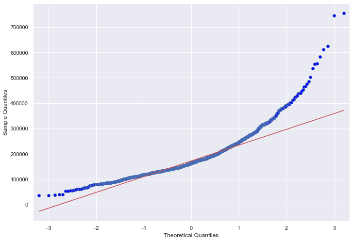
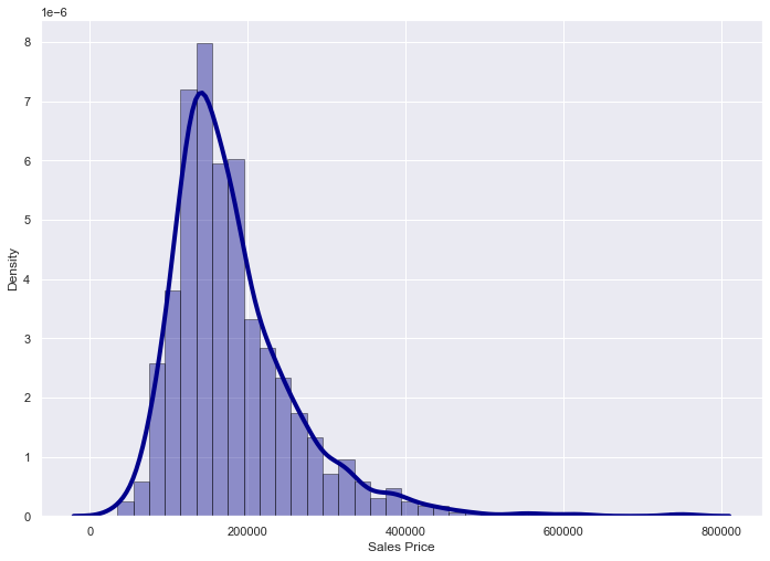
As we can see the QQ-plot seems to have an upwards curvature, this indicates that the data is not linear and and is skewed, this is confirmed when looking at the sale price distribution as it is a right skewed distribution. With this information, we can use a log transformation to transform the dependent variable to achieve a better fit towards a normal distribution.
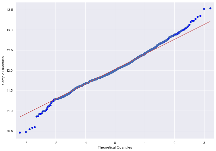
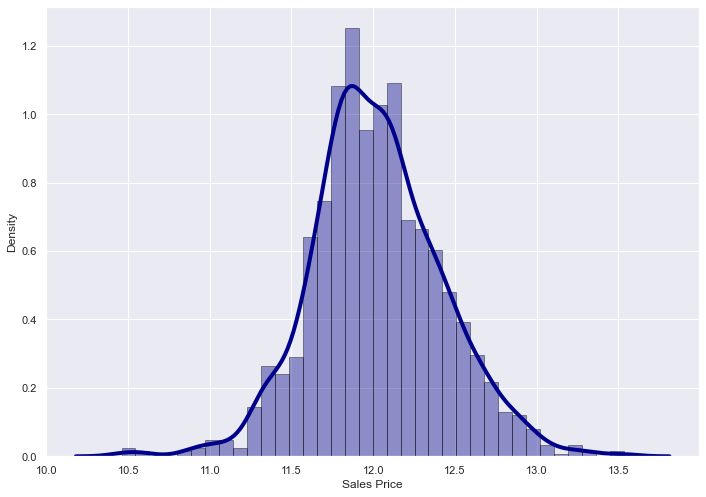
This transformation significantly improved the normality of the sales price. For the time being I will not be investigating the linearity of any of the dependetn variables given the amount of variables that there are. That being said after obtaining a final linear model I will use the obtained variables and ensure that they are all linear.
Analysis
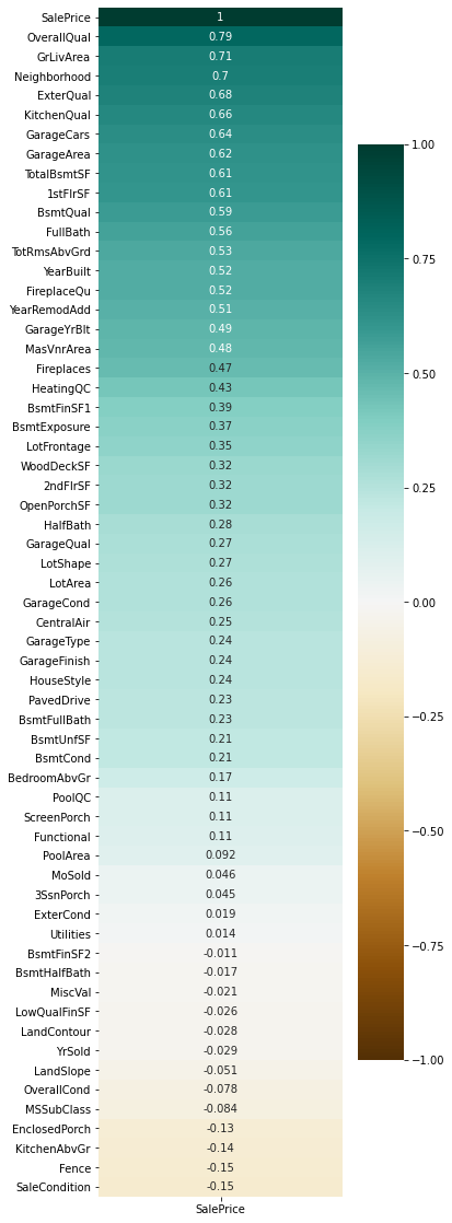
To begin the analysis I first decided to get more insight into the data to better understand the relationships between the dependent variable and the independent variables. To do this I used a correlation matrix that gives an initial understanding of which variables seem to be highly correlated with the sales price. Unsurprisingly the top 3 variables that seem to correlate with sales prices are: Overall quality, neighborhood, and Ground floor living area. These correlations will give us good insight when deciding which variables to keep in case of multi collinearity.
To reduce the number of variables in the final regression I will be using a stepwise backward selection process. Backward selection is done by starting with a regression that includes all variables and systematically removing variables that don't seem to contribute to the regression given their p-value. In this case, my threshold to keep a variable will be set at an alpha = 0.05. Once all variables are below an alpha of 0.05 the stepwise selection will terminate and produce the final model.
After performing a backward selection we got the following variables that seemed to be the most significant in the linear regression:
	OLS Regression Results
	  Dep. Variable:        SalePrice      R-squared (uncentered):         0.973


	  Model:                   OLS         Adj. R-squared (uncentered):    0.972


	  Method:             Least Squares    F-statistic:                    1716.


	  Date:             Sun, 01 Aug 2021   Prob (F-statistic):             0.00


	  Time:                 14:00:50       Log-Likelihood:               -13268.


	  No. Observations:        1121        AIC:                         2.658e+04


	  Df Residuals:            1098        BIC:                         2.670e+04


	  Df Model:                  23


	  Covariance Type:      nonrobust


			          coef     std err      t      P>|t|  [0.025    0.975]


	  Neighborhood  2308.1607   237.480     9.719  0.000  1842.194  2774.127


	  MSSubClass    -190.0565    30.090    -6.316  0.000  -249.097  -131.016


	  LotFrontage   -172.0544    54.509    -3.156  0.002  -279.008   -65.101


	  LotArea          0.4661     0.144     3.234  0.001     0.183     0.749


	  HouseStyle   -4743.8869  2343.042    -2.025  0.043 -9341.232  -146.542


	  OverallQual   1.078e+04  1451.791     7.428  0.000  7934.632  1.36e+04


	  OverallCond   5051.5530  1050.347     4.809  0.000  2990.639  7112.467


	  MasVnrArea      28.6283     6.294     4.549  0.000    16.279    40.977


	  ExterQual     9999.8740  3097.383     3.228  0.001  3922.415  1.61e+04


	  BsmtQual      8313.0791  2205.997     3.768  0.000  3984.634  1.26e+04


	  BsmtCond     -6206.5204  2708.728    -2.291  0.022 -1.15e+04  -891.653


	  BsmtExposure  5674.4909  1178.654     4.814  0.000  3361.822  7987.159


	  BsmtFinSF1      10.2277     3.208     3.188  0.001     3.934    16.522


	  GrLivArea       49.6567     4.416    11.244  0.000    40.992    58.322


	  BsmtFullBath  6130.6166  2691.107     2.278  0.023   850.323  1.14e+04


	  BedroomAbvGr -5939.7076  1912.752    -3.105  0.002 -9692.770 -2186.645


	  KitchenAbvGr -1.792e+04  5946.669    -3.013  0.003 -2.96e+04 -6249.616


	  KitchenQual   1.033e+04  2406.377     4.291  0.000  5603.935   1.5e+04


	  TotRmsAbvGrd  4492.2601  1346.548     3.336  0.001  1850.161  7134.359


	  GarageYrBlt    -72.0393     9.304    -7.743  0.000   -90.294   -53.785


	  GarageCars    1.446e+04  2185.427     6.618  0.000  1.02e+04  1.88e+04


	  GarageQual    9975.0846  3996.579     2.496  0.013  2133.290  1.78e+04


	  ScreenPorch     47.8903    17.782     2.693  0.007    12.999    82.782


	  Omnibus:       376.939   Durbin-Watson:         1.824


	  Prob(Omnibus):  0.000    Jarque-Bera (JB):   49775.782


	  Skew:          -0.407    Prob(JB):               0.00


	  Kurtosis:      35.634    Cond. No.           7.83e+04
The summary of the linear regression gave us a total of 23 highly significant variables that are all below our alpha of 0.05 or 5%. Most of the obtained variables seem to be relatively straight forwards and have logical reasoning behind them such as living area. There are however some peculiar relationships that were uncovered by this analysis. The first that seemed out of place is the variable that accounts for a property having a screen porch. That being said, one possible reasoning behind this could be where the data was obtained(California). Another suspect relationship is the negative relationship lot frontage and sales price has. This seems counterintuitive but on further inspection could be a significant indicator of the size of the house itself. That being said it is still a relatively suspect relationship.
Possible Improvements
The analysis gave a great insight into the factors that seem to contribute most to the sales price of properties in California. That being said there are some things I would like to try to improve the analysis and its accuracy/relevance. The first alteration I would make would be to try and linearize the explanatory variables in the analysis to correct for any nonlinear variables. Additionally, I would like to do a more detailed analysis into the different neighborhoods and living areas and identify the reasonings of their effect on property sales prices.